Lecture 2 – Kinematics and Lorentz Transformations

This is a lecture note of some sections and exercises with some answering attempts which based on Lecture 2 by Vincent Mathieu

Experiments and Frames

Particle kinematics is the application of special relativity to elementary particle reactions. In experiments, the “beam” collides onto the “target” with high energy to create other particles.

Each particle has a 4-vector \(p^{\mu}\):

\[ p^{\mu} = (E, p_x, p_y, p_z) = (E, \vec{p}) \]

Two frames that are commonly used are the Center of Mass (CoM) frame and the laboratory (Lab) frame.

For a two-particle reaction, \(a+b \to 1 + ... + n\), the frames satisfy the following relations.

• Lab frame: \(\vec{p}_b = \vec{0}\)
  Target particle \(b\) is at rest, while beam particle \(a\) is moving.

• CoM frame: \(\vec{p}_a+\vec{p}_b = \vec{0}\)
  The total momentum is zero, i.e., the momenta of the two initial state particles have opposite direction.

Masses can be defined as a Lorentz invariant quantity (unaffected by reference frame):

\[ p^2_i = E^2_i = |\vec{p}_i|^2 = m^2_i \]

where \(p\) is the 4-vector, \(E\) is the energy, \(\vec{p}\) is the three vector, and \(m\) is the mass.

Two particles Final States

Let us now consider the case of a two-body decay (\(n=2\)), i.e., \(a+b \rightarrow 1+2\).

When we have a final state with two particles (\(n=2\)), we can define one \(xz\) plane that is spanned by the momenta of the two final state particles in the Lab frame. The CoM frame and the Lab frame can now be related by a boost along the \(z\)-axis (the direction of particle \(a\)).

With this definition of the \(xz\) plane, we have:

• \(\vec{z}\) is parallel to the beam \(\vec{p}_a\)

• \(\vec{y} \) is parallel to \( \vec{p}_a \times \vec{p}_1\)

Lorentz transformations

Lorentz transformations, can be factorized into rotations and boosts along one axis (or arbitrary direction) and are required for transforming particle properties, such as position and time, between different inertial frames in relative motion.

Boost along one axis

When we boost in the direction of the \(z\) axis, only the energy and the \(z\) component of the four-momenta changes, so we can express the Lorentz boost as a 2D matrix:

\[\begin{split}\begin{pmatrix} E^* \\ p_z^* \end{pmatrix} = \begin{pmatrix} \gamma & \gamma \beta \\ \gamma \beta & \gamma \end{pmatrix} \begin{pmatrix} E^L\\ p^L_z \end{pmatrix}, \end{split}\]

and its inverse relation,

(1)\[\begin{split}\begin{pmatrix} E^L \\ p_z^L \end{pmatrix} = \begin{pmatrix} \gamma & -\gamma \beta \\ -\gamma \beta & \gamma \end{pmatrix} \begin{pmatrix} E^*\\ p^*_z \end{pmatrix}, \end{split}\]

with

(2)\[ \beta = \frac{p^*_b}{m_b} \]

and

(3)\[ \gamma \beta = \frac{E^*_b}{m_b}. \]

Exercise 1

Check that the above boost definition brings the target at rest in the lab frame.

Solution to Exercise 1

From CoM frame to Lab frame, we apply the boost to the 4-vector of particle b (target)

\[\begin{split}\begin{pmatrix} E_b^* \\ p_{b,z}^* \end{pmatrix} = \begin{pmatrix} \gamma & \gamma \beta \\ \gamma \beta & \gamma \end{pmatrix} \begin{pmatrix} E_b^L\\ p^L_{b,z} \end{pmatrix} \end{split}\]

using the relations (2) and (3) and subsititute into (1):

\[ \gamma = \frac{\gamma \beta}{\beta} = \frac{E_b^* m_b}{m_b p_b^*} = \frac{E_b^*}{p_b^*} \]

\[\begin{split}\begin{pmatrix} E_b^L \\ p_{b,z}^L \end{pmatrix} = \begin{pmatrix} \frac{E_b^*}{p_b^*} & -\frac{E_b^*}{m_b} \\ -\frac{E_b^*}{m_b} & \frac{E_b^*}{p_b^*} \end{pmatrix} \begin{pmatrix} E_b^*\\ p^*_{b,z} \end{pmatrix} \end{split}\]

Since it’s only changing in z-componenet and energy, one yields:

\[\begin{split}\begin{pmatrix} E_b^L \\ p_{b,z}^L \end{pmatrix} = % \begin{pmatrix} % \frac{E_b^*}{p_b^*} & -\frac{E_b^*}{m_b} \\ % -\frac{E_b^*}{m_b} & \frac{E_b^*}{p_b^*} % \end{pmatrix} \begin{pmatrix} \frac{E_b^*}{p_{b,z}^*} \cdot E_b^* - \frac{E_b^*}{m_b}p_{b,z}^* \\ -\frac{E_b^*}{m_b} \cdot E_b^* + \frac{E_b^*}{p_{b,z}^*} \cdot p_{b,z}^* \end{pmatrix} \end{split}\]

If particle \(b\) is at rest after inverse-boost, that means the xyz component of momentum of particle \(b\) is zero: \(p_{b,x}^L = p_{b,y}^L = p_{b,z}^L=0\). We have already assume \(p_{b,x}^* = p_{b,y}^* = 0\), and thus \(p_{b,x}^L = p_{b,y}^L = 0\).

In order to have \(p_{b,z}^L=0\), \( p_{b,z}^L = -\frac{E_b^*}{m_b} \cdot E_b^* + \frac{E_b^*}{p_{b,z}^*} \cdot p_{b,z}^* = 0\) must hold.

Therefore, only when \(\frac{E_b^*}{m_b} = 1\) or \(E_b^* = m_b\)

\( \rightarrow p_{b,z}^L =0\). Under this condition, the particle is at rest after inverse-boosted to rest frame.

Rotations

We use active rotations instead of passive rotations. Under an active rotation, the momentum is changed and the axes are fixed

Example: if we rotate a momentum of unit length over the \(z\) axis with an angle \(\theta\), we get:

(4)\[\begin{split} \begin{pmatrix} p_x \\ p_y \\ p_z \end{pmatrix} = \begin{pmatrix} \sin(\theta) \\ 0 \\ \cos(\theta) \end{pmatrix}. \end{split}\]

After a rotation of \(\omega\) around the \(y\) axis, the rotated momentum forms an angle \(\theta + \omega\) with the \(z\) axis, we get:

\[\begin{split} \begin{pmatrix} p_x' \\ p_y' \\ p_z' \end{pmatrix} = R_y(\omega) \begin{pmatrix} p_x \\ p_y \\ p_z \end{pmatrix} = \begin{pmatrix} \sin(\theta+\omega) \\ 0 \\ \cos(\theta+\omega) \end{pmatrix}. \end{split}\]

Exercise 2

Check the result of the rotation above

Solution to Exercise 2

Recall the rotation matrices, any rotation can be decomposed into rotations around \(z\) and \(y\) axes:

\[\begin{split} R_z(\omega) = \begin{pmatrix} \cos(\omega) & -\sin(\omega) & 0 \\ \sin(\omega) & \cos(\omega) & 0 \\ 0 & 0 & 1 \end{pmatrix} \end{split}\]

\[\begin{split} R_y(\omega) = \begin{pmatrix} \cos(\omega) & 0 & \sin(\omega) \\ 0 & 1 & 0 \\ -\sin(\omega) &0 & \cos(\omega) \end{pmatrix} \end{split}\]

The rotation matrix around \(x\) axes is also given for completeness:

\[\begin{split} R_x(\omega) = \begin{pmatrix} 1&0&0 \\ 0 & \cos(\omega) & -\sin(\omega) \\ 0 & \sin(\omega) & \cos(\omega) \end{pmatrix} \end{split}\]

With this, we can rewrite equation (4) as:

\[\begin{split} \begin{pmatrix} p_x' \\ p_y' \\ p_z' \end{pmatrix} = R_y(\omega) \begin{pmatrix} p_x \\ p_y \\ p_z \end{pmatrix} = \begin{pmatrix} \cos(\omega) & 0 & \sin(\omega) \\ 0 & 1 & 0 \\ -\sin(\omega) &0 & \cos(\omega) \end{pmatrix} \begin{pmatrix} p_x \\ p_y \\ p_z \end{pmatrix} \end{split}\]

\[\begin{split} \begin{pmatrix} p_x' \\ p_y' \\ p_z' \end{pmatrix} = \begin{pmatrix} p_x \cdot \cos(\omega)+ p_z \cdot \sin(\omega) \\ p_y \\ -p_x \cdot \sin(\omega) + p_z \cdot \cos(\omega) \end{pmatrix} \end{split}\]

since \(\begin{pmatrix} p_x \\ p_y \\ p_z \end{pmatrix}\) = \(\begin{pmatrix} \sin(\theta) \\ 0 \\ \cos(\theta) \end{pmatrix} \), and using the trigonometric identities, thus we have:

\[\begin{split} \begin{pmatrix} p_x' \\ p_y' \\ p_z' \end{pmatrix} = \begin{pmatrix} \sin(\theta) \cdot \cos(\omega)+ \cos(\theta) \cdot \sin(\omega) \\ 0 \\ -\sin(\theta) \cdot \sin(\omega) + \cos(\theta) \cdot \cos(\omega) \end{pmatrix} = \begin{pmatrix} \sin(\theta+\omega) \\ 0 \\ \cos(\theta+\omega) \end{pmatrix} \end{split}\]

Example with data

Two-particles-1.dat

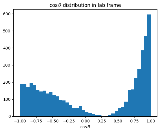
The data are in the lab frame, Compute and plot the \(cosθ_L\) distribution.

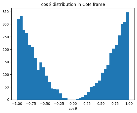
Boost to the CoM and Compute and plot the \(cosθ^*\) distribution

Import Python libraries Hide code cell content

import warnings

import gdown
import numpy as np
from IPython.display import display

warnings.filterwarnings("ignore")

# https://indico.ific.uv.es/event/6803/contributions/21220/attachments/11209/15506/Two-particles-1.dat
filename = gdown.cached_download(
    url="https://indico.ific.uv.es/event/6803/contributions/21220/attachments/11209/15506/Two-particles-1.dat",
    path="data/Two-particles-1.dat",
    md5="324f71ee88928915f13de5840ac5ede2",
    quiet=True,
    verify=False,
)
data = np.loadtxt(filename)
data.shape

(15000, 4)

# 4-vector for a+b->1+2
pa = data[::3].T
p1 = data[1::3].T
p2 = data[2::3].T
pa.shape

(4, 5000)

# 4-vector conservation
pb = p1 + p2 - pa
assert pb.std(axis=1).sum().round(5) == 0
pb.mean(axis=1).round(3)

array([ 0.938,  0.   ,  0.   , -0.   ])

m1 = np.sqrt(p1[0] ** 2 - p1[1] ** 2 - p1[2] ** 2 - p1[3] ** 2)
m1.mean(), m1.std()

(0.13999997797061128, 9.590363480890062e-07)

# p1.shape
np.sqrt((p1[1:] ** 2).sum(axis=0))

array([0.19442312, 0.17937091, 0.13473493, ..., 0.20285078, 0.19812602,
       0.18215134])

because this decay happend in x-z plane, thus we can find the \(\cos \theta\) by:

(5)\[ \cos \theta = \frac{p_{1z}}{|\vec{p_1}|} \]

def p3_length(four_momentum: np.ndarray) -> np.ndarray:
    return np.sqrt(
        four_momentum[1] ** 2 + four_momentum[2] ** 2 + four_momentum[3] ** 2
    )


p1_length = p3_length(p1)
cos_theta = p1[3] / p1_length

Show code cell source Hide code cell source

p1_length_vectorized = np.sqrt(np.sum(p1[1:] ** 2, axis=0))
np.testing.assert_array_equal(p1_length, p1_length_vectorized)

Show code cell source Hide code cell source

import matplotlib.pyplot as plt

# cos(theta) in lab frame
plt.title(r"$\cos \theta$ distribution in lab frame")
plt.xlabel(r"$\cos \theta$")
plt.hist(cos_theta, bins=40)
plt.show()

cos \(\theta\) in CoM frame

Performing boost from calculation via numpy

The total initial 4-momentum in the lab frame is given by:

\[ \vec{P} = \vec{p}_a + \vec{p}_b \]

# The total initial 4-momentum in lab frame
p_CM_lab = pa + pb

Total Energy in CM frame is the magnitude of the total initial 4-momentum:

\[ E_{CM} = \sqrt{\vec{P} \cdot \vec{P}} = \sqrt{(E_a+m_b)^2 - |\vec{p_a}|^2} = \sqrt{s} \]

This is valid, as we know that \(\sqrt{s}\) is the total energy in CoM frame of the colliding particles, in this case: for two particle final state of reaction \(a+b \rightarrow 1+2\)

\[ E_{CM} = \sqrt{s} = \sqrt{(E_a+E_b)^2 - |\vec{p_a} + \vec{p_b}|^2} = \sqrt{(E_a+m_b)^2 - |\vec{p_a}|^2} \]

pa_length = p3_length(pa)
E_CM = np.sqrt(p_CM_lab[0] ** 2 - pa_length**2)

E_CM_lab = p_CM_lab[0]
βx_CM, βy_CM, βz_CM = β_CM = pa[1:] / E_CM_lab
β2 = βx_CM**2 + βy_CM**2 + βz_CM**2
gamma = 1 / np.sqrt(1 - β2)

Find the transformed energy \(E_1\) in CoM frame by Lorentz boost for \(p^{0}_1\) :

\[ E_{1,CM} = \gamma(E_1 - \vec{\beta} \cdot \vec{p}_1) \]

where

\[ \gamma = \frac{1}{\sqrt{1-\beta^2}} \]

and \(\beta\) is the velocity here

E1_CM = gamma * (p1[0] - βx_CM * p1[1] - βy_CM * p1[2] - βz_CM * p1[3])

And now for the transformed momentum vector \(\vec{p}_1\) in CoM frame by Lorentz boost for \(p_1^{i}\), where i = 1,2,3, with:

\[ \vec{p}_{1,CM} = \vec{p}_1 + (\frac{\gamma -1}{\beta^2}(\vec{\beta} \cdot \vec{p}_1)- \gamma E_1) \vec{\beta} \]

p1_vec = p1[1:]
f = β_CM * p1_vec
f1 = (gamma - 1) / β2
f2 = gamma * p1[0]
p1_CM_vec = p1_vec + (f1 * f - f2) * β_CM

p1_CM = np.concatenate((E1_CM[None], p1_CM_vec))
p1_CM

array([[ 0.28822499,  0.20354655,  0.21832548, ...,  0.27259354,
         0.25480815,  0.26263327],
       [ 0.087408  , -0.056301  ,  0.064965  , ...,  0.12147   ,
        -0.184504  ,  0.124774  ],
       [ 0.088406  ,  0.007849  ,  0.013297  , ..., -0.144377  ,
         0.067113  ,  0.071142  ],
       [-0.21912947,  0.13638077, -0.15384603, ..., -0.13823006,
        -0.08234951, -0.16954799]])

Similarily, the equation (5) is still hold, and thus we find the \(\cos \theta_{CM}\):

p1_CM_length = p3_length(p1_CM)
cos_theta_CM = -p1_CM[3] / p1_CM_length

Show code cell source Hide code cell source

plt.hist(cos_theta_CM, bins=40)
plt.title(r"$\cos \theta$ distribution in CoM frame")
plt.xlabel(r"$\cos \theta$")
plt.show()

Perfroming boost using pylorentz package below to test the boost again:

Show code cell source Hide code cell source

from pylorentz import Momentum4

p1_Lab = Momentum4(*p1)
pa_Lab = Momentum4(*pa)
pb_Lab = Momentum4(*pb)
p2_Lab = Momentum4(*p2)

cm = pa_Lab + pb_Lab
p1_CM_pyL = p1_Lab.boost_particle(-cm)

cos_theta_CM_pyL = p1_CM_pyL.p_z / p1_CM_pyL.p

# check the cos theta CM in 2 different ways
np.testing.assert_allclose(cos_theta_CM, cos_theta_CM_pyL, rtol=1e-5)
print("test past with relative tolerance 1e-5")

test past with relative tolerance 1e-5

Show code cell content Hide code cell content

plt.hist(cos_theta_CM_pyL, bins=40)
plt.title(r"$\cos \theta$ distribution in CoM frame")
plt.xlabel(r"$\cos \theta$")
plt.show()

Mandelstam variables

We have the mass-shell relation:

\[ p_i^2 = m^2_i \]

The Mandelstam variables s, t, and u are Lorentz invariants. Their definition are:

\[ s =(p_a + p_b)^2 = (p_1+p_2)^2 \]

\[ t =(p_a - p_1)^2 = (p_b-p_2)^2 \]

\[ u =(p_a - p_2)^2 = (p_b-p_1)^2 \]

(6)\[ s+t+u = m_a^2+m_b^2+m_1^2+m^2_2 \]

Exercise 3

Check the relation in equation (6) by using \(p_a+p_b=p_1+p_2\)

Solution to Exercise 3

\[ s+t+u = (p_a + p_b)^2 + (p_a - p_1)^2 + (p_a - p_2)^2\]

\[ s+t+u = p_a^2 +p_b^2 + 2 p_a p_b + p_a^2 -2 p_a p_1 + p_1^2 + p_a^2 - 2p_a p_2 +p_2^2\]

(7)\[ s+t+u = 3p_a^2 + p_b^2 +p_1^2 + p_2^2 + 2p_a p_b - 2p_a p_1 -2 p_a p_2 \]

from equation (6) we have:

\[ p_b = p_1 + p_2 - p_a \]

(8)\[ p_a \cdot p_b = p_a \cdot p_1 + p_a \cdot p_2 - p_a^2 \]

By equation (7) and substitute it into equation (8):

\[ s+t+u = 3p_a^2 + p_b^2 +p_1^2 + p_2^2 + 2p_a \cdot p_1 + 2p_a \cdot p_2 - 2p_a^2 -2p_a p_1 -2 p_a p_2 \]

\[ s+t+u = p_a^2 + p_b^2 +p_1^2 + p_2^2 \]

by the mass shell relation, and thus:

\[s+t+u = m_a^2 + m_b^2 + m_1^2 + m_2^2\]

CoM Kinematics

Every frame dependent quantities is expressed with Mandelstam variables

\(p_a = (E_a^*,0,0,|\vec{p_a}^*|)\)

\(p_b = (E_b^*,0,0,-|\vec{p_a}^*|)\)

\(p_1 = (E_1^*, |\vec{p_1}^*|sin \theta^*,0, |\vec{p_1}^*|cos \theta^*)\)

\(p_2 = (E_2^*, -|\vec{p_1}^*| sin \theta^*,0, -|\vec{p_1}^*|cos \theta^*)\)

Invariant: $\(s = (p_a + p_b)^2 = (E_a^* + E_b^*)^2 = E_{CM}^2\)$

\[ t = (p_a - p_1)^2 = m_a^2 + m_1^2 - 2E_a^* E_1^* + 2 |\vec{p_a}^*| |\vec{p_1}^*| cos \theta^*\]

\(p_1^2 = [ (p_a+p_b) - p_2 ]^2\)

Exercise 4

Check that \(E_1^* = \frac{s+m^2_1-m_2^2}{2 \sqrt{s}}\) and \(E_2^* = \frac{s+m^2_2-m_1^2}{2 \sqrt{s}}\)

Solution to Exercise 4

\[ E_2^* = E_a^* + E_b^* - E_1^* = E^*_{CM} - E_1^* = \sqrt{s} - E_1^* = \sqrt{s} - \sqrt{\vec{p_1}^2 + m_1^2} \]

\[ E_2^{*2} = s + \vec{p_1}^2 + m_1^2 - 2\sqrt{s}\sqrt{\vec{p}^2+m_1^2} \]

\[ E_2^{*2} = \vec{p_1}^2 + m_2^2 \]

from the 2 equations of \(E_2^{*2}\) above, we have: $\( s + \vec{p_1}^2 + m_1^2 - 2\sqrt{s}\sqrt{\vec{p}^2+m_1^2} = \vec{p_1}^2 + m_2^2 \)$

\[ s + m_1^2 - 2\sqrt{s}\sqrt{\vec{p}^2+m_1^2} = m_2^2 \]

\[ s + m_1^2 - m_2^2 = 2\sqrt{s}E_1^* \]

We have E_1^* : $\( E_1^* = \frac{s + m_1^2 - m_2^2 }{2\sqrt{s}} \)$

For E_2^* : $\( E_2^* = \sqrt{s} - E_1^* = \sqrt{s} - \frac{s + m_1^2 - m_2^2 }{2\sqrt{s}} = \frac{s + m_2^2 - m_1^2 }{2\sqrt{s}} \)$

Exercise 5

Check that \(|\vec{p_1}^*| = \sqrt{(E_1*)^2-m_1^2} = \frac{\lambda^{1/2}(s,m_1^2,m_2^2)}{2 \sqrt{s}}\), where \(\lambda(a,b,c) = a^2+b^2+c^2 - 2(ab+bc+ca)\)

Solution to Exercise 5

\[ t_{min,max} = m_a^2 + m_1^2 - 2E_a^* E_1^* + 2 |\vec{p_a}^*| |\vec{p_1}^*| \]

Equivalent expression for the scattering angle in the CoM

\[ cos \theta^* = 1 + \frac{t-t_{min}}{2|\vec{v}_a^*||\vec{p}_1^*|} = \frac{s(t-u)+(m_a^2-m-b^2)(m_1^2-m_2^2)}{\lambda^{1/2}(s,m_a^2,m_b^2)\lambda^{1/2}(s,m_1^2,m_2^2)} \]

Compute \(cos \theta^L\) as a function of s,t,u

\[ cos \theta^L \]

Three particles final states

Relevant Variables

Reference Frames

For scattering study in 3 body final states, the Gottfried-Jackson frame and the helicity frame are two different particular center-of-mass reference frames used to analyze the angular distribution and polarization of particles in high-energy physics experiments, they are particularly useful in the study of scattering processes.

Gottfried-Jackson and helicity frames are related by a rotation of angle ω around y

Gottfried-Jackson Frame

It is particularly useful when the particles involved have non-zero spin, and their spin orientations are aligned with their motion, making the analysis of their angular distributions relative to their spin directions more straightforward

Helicity Frame

This frame is often used in the analysis of the decay products of a particle, where it’s important to understand the spin orientation relative to the direction of motion.

Decay into two particles

Decay into three particles

\[\theta^*_{12}+\theta^*_{23}+\theta^*_{31}=2 \pi\]

Dalitz Plot

Exercise: Three-particles-1.dat

Lecture 2 by Vincent Mathieu contains a few data files containing four-momenta data samples. Our goal in this notebook is to identify which reaction was used to generate these data samples.

Exercise 6

File: Three-Particles-1.dat is The data are in the lab frame, with Format:

Ea, pa,x, pa,y, pa,z

E1, p1,x, p1,y, p1,z

E2, p2,x, p2,y, p2,z

E3, p3,x, p3,y, p3,z

. . . .

. . . .

. . . .

Three questions to be found out.

Which reaction is it?

What resonances are included?

What is the spin of the resonances?

Solution to Exercise 6

filename = gdown.cached_download(
    url="https://indico.ific.uv.es/event/6803/contributions/21220/attachments/11209/15504/Three-particles-1.dat",
    path="data/Three-particles-1.dat",
    md5="a49ebfd97ae6a02023291df665ab924c",
    quiet=True,
    verify=False,
)
data = np.loadtxt(filename)
data.shape

(400000, 4)

print(data)

[[ 1.943718  0.        0.        1.943718]
 [ 1.061417  0.754321  0.202865  0.464916]
 [ 1.113291 -0.15559   0.010675  1.094015]
 ...
 [ 1.943001  0.038062 -0.0882    1.861644]
 [ 0.225227 -0.031795 -0.03032  -0.174848]
 [ 1.933704 -0.006267  0.11852  -1.686797]]

n_final_state = 3
pa, p1, p2, p3 = (data[i::4].T for i in range(n_final_state + 1))
p0 = p1 + p2 + p3
pb = p0 - pa

def mass(p: np.ndarray) -> np.ndarray:
    return np.sqrt(mass_squared(p))


def mass_squared(p: np.ndarray) -> np.ndarray:
    return p[0] ** 2 - np.sum(p[1:] ** 2, axis=0)


m0 = mass(p0)
print(f"{m0.mean():.4g} +/- {m0.std():.4g}")

4.102 +/- 4.992e-07

Show code cell source Hide code cell source

from IPython.display import Math

display(Math(Rf"m_a = {mass(pa).mean():.3g}\text{{ GeV}}"))
display(Math(Rf"m_b = {mass(pb).mean():.3g}\text{{ GeV}}"))
for i, p in enumerate([p0, p1, p2, p3]):
    display(Math(Rf"m_{i} = {mass(p).mean():.3g}\text{{ GeV}}"))

\[\displaystyle m_a = 0\text{ GeV}\]

\[\displaystyle m_b = 0.938\text{ GeV}\]

\[\displaystyle m_0 = 4.1\text{ GeV}\]

\[\displaystyle m_1 = 0.548\text{ GeV}\]

\[\displaystyle m_2 = 0.135\text{ GeV}\]

\[\displaystyle m_3 = 0.938\text{ GeV}\]

Identify final state particles Hide code cell source

from particle import Particle


def find_candidates(
    mass: float, delta: float = 0.001, charge: float | None = None
) -> list[Particle]:
    def identify(p) -> bool:
        if p.pdgid in {21}:
            return
        if charge is not None and p.charge != charge:
            return False
        if (mass - delta) < 1e-3 * p.mass < (mass + delta):
            return True
        return False

    return Particle.findall(identify)


ma = mass(pa).mean()
mb = mass(pb).mean()
m1 = mass(p1).mean()
m2 = mass(p2).mean()
m3 = mass(p3).mean()
initial_state = (
    find_candidates(ma.mean(), delta=1e-4)[0],
    find_candidates(mb.mean())[0],
)
final_state = tuple(find_candidates(m.mean())[0] for m in [m1, m2, m3])
display(
    Math(R"\text{Incoming: }" + ", ".join(f"{p.latex_name}" for p in initial_state)),
    Math(R"\text{Outgoing: }" + ", ".join(f"{p.latex_name}" for p in final_state)),
)

\[\displaystyle \text{Incoming: }\gamma, p\]

\[\displaystyle \text{Outgoing: }\eta, \pi^{0}, p\]

So this is a photon \(\gamma\) hitting a proton \(p\) and producing a meson \(\eta\), pion \(\pi^0\), and proton \(p\).

Dalitz plot

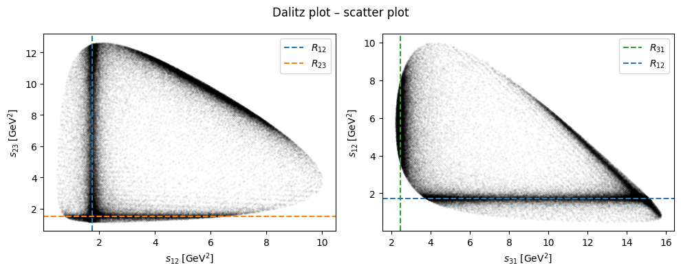
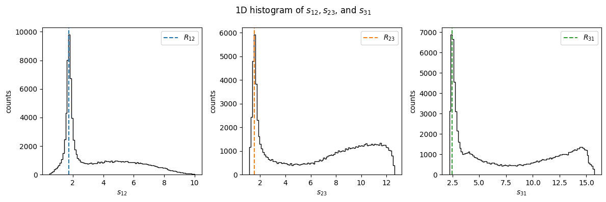
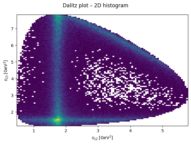
By plotting the three Mandelstam variables in a Dalitz plot, we can identify resonances appear in the reaction for which this data was generated.

s12 = mass_squared(p1 + p2)
s23 = mass_squared(p2 + p3)
s31 = mass_squared(p3 + p1)

m12 = mass(p1 + p2)
m23 = mass(p2 + p3)
m31 = mass(p3 + p1)

Show code cell source Hide code cell source

import matplotlib.pyplot as plt

fig, ax = plt.subplots()
fig.suptitle("Dalitz plot – 2D histogram")
ax.hist2d(s12, s23, bins=100, cmin=1)
ax.set_xlabel(R"$s_{12}\;\left[\mathrm{GeV}^2\right]$")
ax.set_ylabel(R"$s_{23}\;\left[\mathrm{GeV}^2\right]$")
fig.tight_layout()
plt.show()

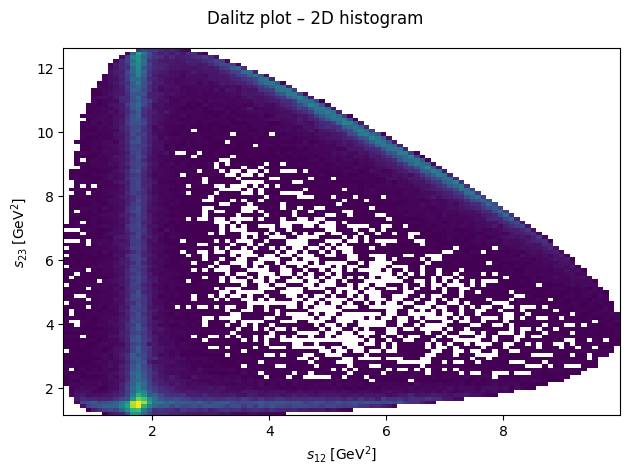
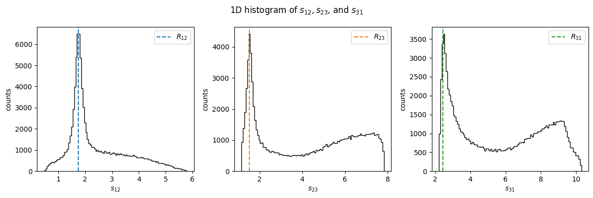
R12 = 1.74
R23 = 1.53
R31 = 2.45

Show code cell source Hide code cell source

fig, (ax1, ax2) = plt.subplots(figsize=(10, 4), ncols=2)
fig.suptitle("Dalitz plot – scatter plot")
ax1.scatter(s12, s23, c="black", s=1e-3)
ax1.set_xlabel(R"$s_{12}\;\left[\mathrm{GeV}^2\right]$")
ax1.set_ylabel(R"$s_{23}\;\left[\mathrm{GeV}^2\right]$")
ax1.axvline(R12, c="C0", ls="dashed", label="$R_{12}$")
ax1.axhline(R23, c="C1", ls="dashed", label="$R_{23}$")
ax1.legend()
ax2.scatter(s31, s12, c="black", s=1e-3)
ax2.set_xlabel(R"$s_{31}\;\left[\mathrm{GeV}^2\right]$")
ax2.set_ylabel(R"$s_{12}\;\left[\mathrm{GeV}^2\right]$")
ax2.axvline(R31, c="C2", ls="dashed", label="$R_{31}$")
ax2.axhline(R12, c="C0", ls="dashed", label="$R_{12}$")
ax2.legend()
fig.tight_layout()
plt.show()

Show code cell source Hide code cell source

fig, (ax1, ax2, ax3) = plt.subplots(figsize=(12, 4), ncols=3)
fig.suptitle("1D histogram of $s_{12}, s_{23}$, and $s_{31}$")
ax1.hist(s12, bins=100, color="black", histtype="step")
ax1.set_xlabel(R"$s_{12}$")
ax1.set_ylabel("counts")
ax1.axvline(R12, c="C0", ls="dashed", label="$R_{12}$")
ax1.legend()

ax2.hist(s23, bins=100, color="black", histtype="step")
ax2.set_xlabel(R"$s_{23}$")
ax2.set_ylabel("counts")
ax2.axvline(R23, c="C1", ls="dashed", label="$R_{23}$")
ax2.legend()

ax3.hist(s31, bins=100, color="black", histtype="step")
ax3.set_xlabel(R"$s_{31}$")
ax3.set_ylabel("counts")
ax3.axvline(R31, c="C2", ls="dashed", label="$R_{31}$")
ax3.legend()

fig.tight_layout()
plt.show()

Particle identification

In the following, we make a few cuts on Mandelstam variables to select a region where the resonances lie isolated. We then use these cuts as a filter on the computed masses for each each and then compute the mean.

m12_mean = m12[(s12 < 3) & (2.5 < s23) & (s23 < 10)].mean()
m12_mean**2

1.7290722578143247

m23_mean = m23[s23 < 2.5].mean()
m23_mean**2

1.6561439882106896

m31_mean = m31[(s12 > 3) & (s31 < 4)].mean()
m31_mean**2

2.692708758538996

The particle candidates for \(R_{12} \to \eta\pi^0\), \(R_{23} \to \pi^0 p\), and \(R_{31} \to p\eta\) are then:

find_candidates(mass=np.sqrt(R12), delta=0.01, charge=0)

[<Particle: name="a(2)(1320)0", pdgid=115, mass=1318.2 ± 0.6 MeV>,
 <Particle: name="Xi0", pdgid=3322, mass=1314.86 ± 0.20 MeV>,
 <Particle: name="Xi~0", pdgid=-3322, mass=1314.86 ± 0.20 MeV>]

find_candidates(mass=np.sqrt(R23), delta=0.01, charge=+1)

[<Particle: name="Delta(1232)~+", pdgid=-1114, mass=1232.0 ± 2.0 MeV>,
 <Particle: name="Delta(1232)+", pdgid=2214, mass=1232.0 ± 2.0 MeV>,
 <Particle: name="b(1)(1235)+", pdgid=10213, mass=1230 ± 3 MeV>,
 <Particle: name="a(1)(1260)+", pdgid=20213, mass=1230 ± 40 MeV>]

find_candidates(mass=np.sqrt(R31), delta=0.01, charge=+1)

[<Particle: name="Delta(1600)~+", pdgid=-31114, mass=1570 ± 70 MeV>,
 <Particle: name="Delta(1600)+", pdgid=32214, mass=1570 ± 70 MeV>]

Exercise: Three-particles-2.dat

Exercise 7

File: Three-Particles-2.dat is also The data are in the lab frame, with Format:

Ea, pa,x, pa,y, pa,z

E1, p1,x, p1,y, p1,z

E2, p2,x, p2,y, p2,z

E3, p3,x, p3,y, p3,z

. . . .

. . . .

. . . .

Three questions to be found out.

Which reaction is it?

What resonances are included?

What is the spin of the resonances?

Load data Hide code cell content

filename2 = gdown.cached_download(
    url="https://indico.ific.uv.es/event/6803/contributions/21220/attachments/11209/15511/Three-particles-2.dat",
    path="data/Three-particles-2.dat",
    md5="831aee9fd925c43e8630edc6783ab28d",
    quiet=True,
    verify=False,
)
data2 = np.loadtxt(filename2)
pa, p1, p2, p3 = (data2[i::4].T for i in range(n_final_state + 1))

p0 = p1 + p2 + p3
m0 = mass(p0)
print(f"{m0.mean():.4g} +/- {m0.std():.4g}")

3.346 +/- 4.992e-07

Show code cell source Hide code cell source

from IPython.display import Math

for i, p in enumerate([p0, p1, p2, p3]):
    display(Math(Rf"m_{i} = {mass(p).mean():.3g}\text{{ GeV}}"))

display(Math(Rf"m_{{a}} = {mass(pa).mean():.3g}\text{{ GeV}}"))

\[\displaystyle m_0 = 3.35\text{ GeV}\]

\[\displaystyle m_1 = 0.548\text{ GeV}\]

\[\displaystyle m_2 = 0.135\text{ GeV}\]

\[\displaystyle m_3 = 0.938\text{ GeV}\]

\[\displaystyle m_{a} = 0\text{ GeV}\]

Identify final state particles Hide code cell source

from particle import Particle


def find_candidates(m: float, delta: float = 0.001) -> list[Particle]:
    return Particle.findall(lambda p: (m - delta) < 1e-3 * p.mass < (m + delta))


m1 = mass(p1).mean()
m2 = mass(p2).mean()
m3 = mass(p3).mean()
particles = tuple(find_candidates(m.mean())[0] for m in [m1, m2, m3])

src = R"\text{Final state: }" + ", ".join(f"{p.latex_name}" for p in particles)
Math(src)

\[\displaystyle \text{Final state: }\eta, \pi^{0}, p\]

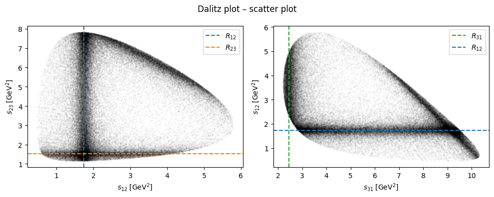
This is again a photon \(\gamma\) hitting a target that produces a meson \(\eta\), pion \(\pi^0\), and proton \(p\).

s12 = mass_squared(p1 + p2)
s23 = mass_squared(p2 + p3)
s31 = mass_squared(p3 + p1)

m12 = mass(p1 + p2)
m23 = mass(p2 + p3)
m31 = mass(p3 + p1)

Show code cell source Hide code cell source

import matplotlib.pyplot as plt

fig, ax = plt.subplots()
fig.suptitle("Dalitz plot – 2D histogram")
ax.hist2d(s12, s23, bins=100, cmin=1)
ax.set_xlabel(R"$s_{12}\;\left[\mathrm{GeV}^2\right]$")
ax.set_ylabel(R"$s_{23}\;\left[\mathrm{GeV}^2\right]$")
fig.tight_layout()
plt.show()

Show code cell source Hide code cell source

fig, (ax1, ax2) = plt.subplots(figsize=(10, 4), ncols=2)
fig.suptitle("Dalitz plot – scatter plot")
ax1.scatter(s12, s23, c="black", s=1e-3)
ax1.set_xlabel(R"$s_{12}\;\left[\mathrm{GeV}^2\right]$")
ax1.set_ylabel(R"$s_{23}\;\left[\mathrm{GeV}^2\right]$")
ax1.axvline(R12, c="C0", ls="dashed", label="$R_{12}$")
ax1.axhline(R23, c="C1", ls="dashed", label="$R_{23}$")
ax1.legend()
ax2.scatter(s31, s12, c="black", s=1e-3)
ax2.set_xlabel(R"$s_{31}\;\left[\mathrm{GeV}^2\right]$")
ax2.set_ylabel(R"$s_{12}\;\left[\mathrm{GeV}^2\right]$")
ax2.axvline(R31, c="C2", ls="dashed", label="$R_{31}$")
ax2.axhline(R12, c="C0", ls="dashed", label="$R_{12}$")
ax2.legend()
fig.tight_layout()
plt.show()

Show code cell source Hide code cell source

fig, (ax1, ax2, ax3) = plt.subplots(figsize=(12, 4), ncols=3)
fig.suptitle("1D histogram of $s_{12}, s_{23}$, and $s_{31}$")
ax1.hist(s12, bins=100, color="black", histtype="step")
ax1.set_xlabel(R"$s_{12}$")
ax1.set_ylabel("counts")
ax1.axvline(R12, c="C0", ls="dashed", label="$R_{12}$")
ax1.legend()

ax2.hist(s23, bins=100, color="black", histtype="step")
ax2.set_xlabel(R"$s_{23}$")
ax2.set_ylabel("counts")
ax2.axvline(R23, c="C1", ls="dashed", label="$R_{23}$")
ax2.legend()

ax3.hist(s31, bins=100, color="black", histtype="step")
ax3.set_xlabel(R"$s_{31}$")
ax3.set_ylabel("counts")
ax3.axvline(R31, c="C2", ls="dashed", label="$R_{31}$")
ax3.legend()

fig.tight_layout()
plt.show()